Comparing classifiers via bootstrapped confidence intervals

If we have two classifiers to perform the same task, how can we tell, which one is better? We could, of course, compare their accuracy: If the first classifier has an accuracy of 70% and the second classifier has an accuracy of 72%, then clearly the second classifier better, right? Well, maybe…

The use of accuracy in this article is a conscious simplification. In many applications, we care about other metrics in addition to, or instead of accuracy, such as: type I and type II errors, differences in error rates between subsets of data, non-regression on certain samples, etc. The principles for comparing classifiers via joint vs. independent sampling, discussed here in the context of accuracy, remain applicable to most other metrics.

Confidence intervals

We have measured accuracies of 70% and 72% on a held out test set. But what we are really interested in, is the accuracy of the classifier when it is deployed in its intended application. The test set accuracy is only a point measurement of the underlying true accuracy. And since every point measurement comes with uncertainty we should attempt to quantify the uncertainty. One possibility to quantify uncertainty is via confidence intervals (CIs).

For accuracy, we have two ways of computing confidence intervals. We can treat the evaluation of the classifier of the test set as a bernoulli random variable \(X\), where for a sample \(x_i=1\), if the classifier correctly classifies \(x_i\), and \(x_i=0\) otherwise. Then the accuracy of the classifier corresponds to the success probability \(P(X=1)\) and there are well-established methods to calculate confidence intervals for the success probability of a bernoulli random variable.

Bootstrapping

A more general method to compute CIs that is applicable to any measurement is bootstrapping. Let us assume that we have a dataset \(\mathbf{x} = (x_1, \ldots, x_n)\) and a metric \(m(\mathbf{x})\) for which we want to compute confidence intervals. We do the following:

• From our dataset \(\mathbf{x} = (x_1, \ldots, x_n)\), we sample with replacement a new dataset \(\mathbf{x'} = (x'_1, \ldots, x'_n)\) of the same size and we compute the metric \(m(\mathbf{x}')\) on the sampled dataset;
• We repeat the process \(N\) times (usually \(N=1,\!000\)) and obtain \(N\) measurements of the metric \((m_1, \ldots, m_N)\);
• The 95%-CI for \(m(\mathbf{x})\) is given by the 2.5%- and 97.5%-quantiles of the set of bootstrapped measurements \(\mathbf{x'} = (x'_1, \ldots, x'_n)\).

The beauty of this procedure is that while we will apply it to the accuracy or the difference of two accuracies, it can be applied without change to any metric \(m\) computed from a dataset. No assumptions on the distribution of the dataset or \(m\) are necessary.¹

Confidence interval width

Before we look at comparing classifiers, we should take a look at the factors influencing the width of confidence intervals. There are two main factors:

• Acuracy of the classifier and
• Size of the dataset.

To better understand the impact of each, it is helpful to convert accuracy to its complement, error rate, \(\mathrm{Err} = 1 - \mathrm{Acc}\) and to think of dataset size in terms of the support of the error rate, i.e., how many incorrectly classified samples we have in the dataset,

\[\mathrm{Support} = n \cdot \mathrm{Err}\,.\]

For example

• With a dataset of size 1,000, a 90% accurate classifier would have support 100.
• Similarly, with a dataset of size 10,000, a 99% accurate classifier would also have support 100.

The diagram shows the size of confidence intervals for classifiers with varying error rates on datasets with varying support.

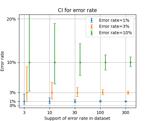
Width of confidence intervals for different classifier accuracies and dataset supports.

However, if we plot the same graph with a logarithmic \(y\)-axis, structure becomes apparent.

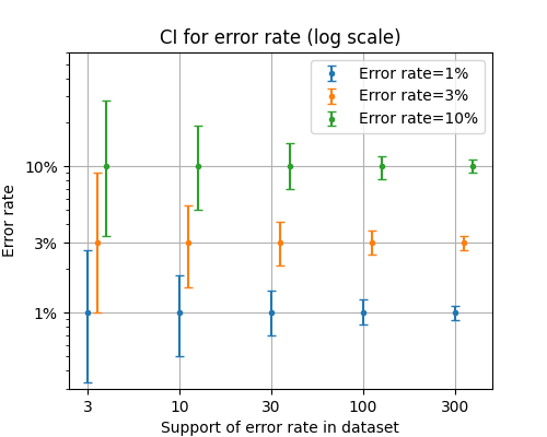
Width of confidence intervals for different classifier accuracies and dataset supports at log scale.

The relative size of confidence intervals, depends only on the size of the support and not on the accuracy of the classifier; i.e., for a CI \((\theta_-, \theta_+)\) around a measurement \(\widehat \theta\), its relative size is \((\theta_+ - \theta_-) / \widehat \theta\). We see in the plot above that the relative size of the CIs does not depend on the absolute accuracy of the classifier and is only a function of the dataset support.²

Comparing classifiers

Let’s come back to the problem of comparing classifiers. We want to account for measurement uncertainty and distinguish, whether we are confident that the second classifier is better than the first one, or whether us measuring 72% accuracy compared to 70% accuracy on the test set was likely down to chance.

We will do this by looking at confidence intervals for the difference in accuracy, i.e., for a dataset \(\mathbf{x}=(x_1, ..., x_n)\), we consider the function \(\Delta \mathrm{Acc}(\mathbf{x}) = \mathrm{Acc}_2(\mathbf{x}) - \mathrm{Acc}_1(\mathbf{x})\) and we bootstrap confidence intervals for \(\Delta \mathrm{Acc}\).

If the confidence interval does not intersect 0, then we can be 95%-confident that the second classifier is indeed better than the first one.

Independent sampling

How do we arrive at a confidence interval for \(\Delta \mathrm{Acc}\). We know how to compute confidence intervals for \(\mathrm{Acc}_1\) and \(\mathrm{Acc}_2\) via bootstrapping, so we could follow a similar process.

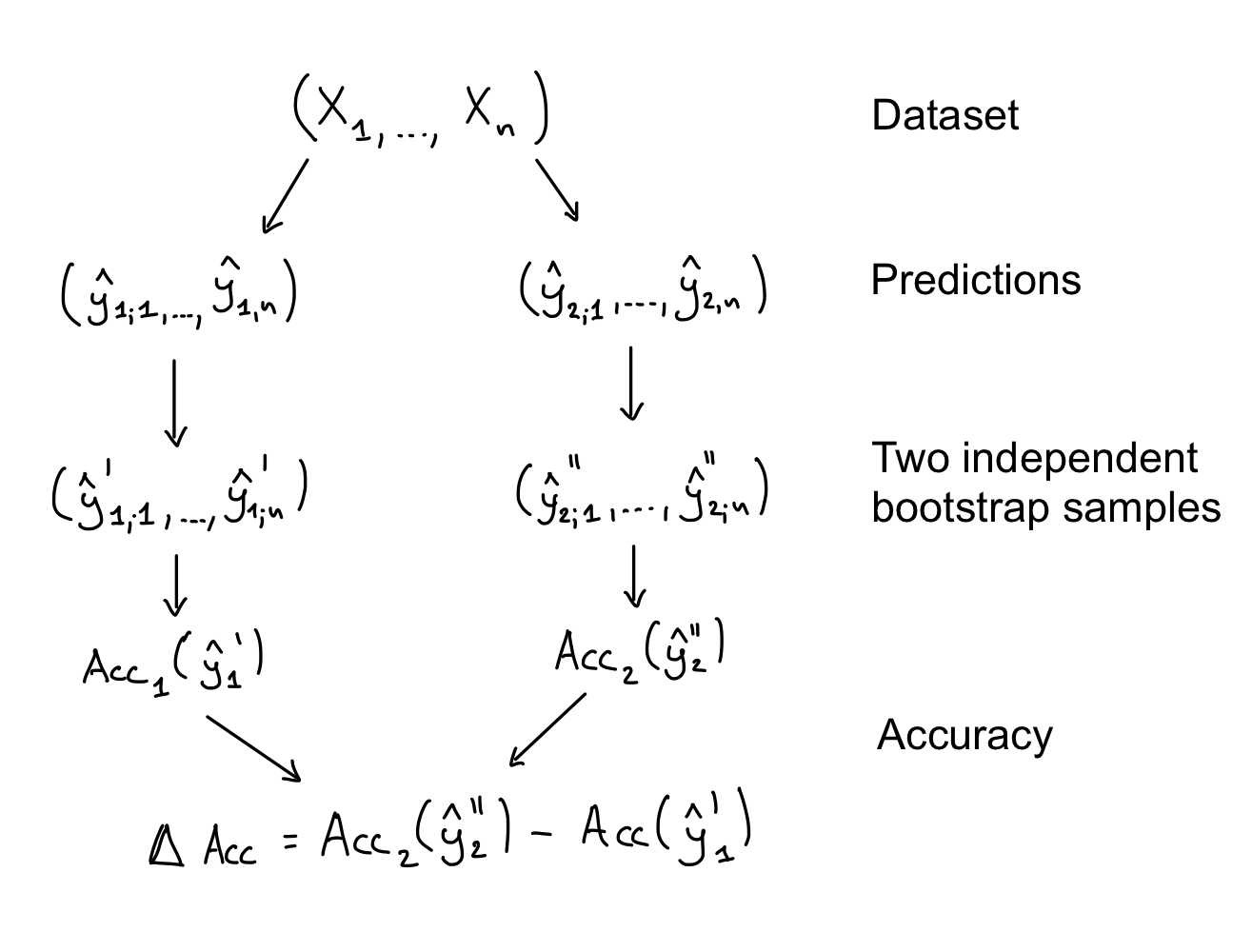
Bootstrapping for \(\Delta \mathrm{Acc}\) via independent sampling.

In this procedure we compute independent bootstrap samples \((\mathrm{Acc}_1(\mathbf{x}'_1), ..., \mathrm{Acc}_1(\mathbf{x}'_N))\) and \((\mathrm{Acc}_1(\mathbf{x}''_2, ..., \mathrm{Acc}_1(\mathbf{x}''_N))\) for each accuracy before taking their difference. In general, however, this will lead to too wide confidence intervals, because it ignores any possible correlation between the two classifiers and their predictions.

Correlation between classifiers

Why should we expect the predictions of two classifiers to be correlated? If the two classifiers are based on different model architectures, and if they have been trained on different datasets, then it is indeed possible that their results will be uncorrelated. But usually, work on an ML model is iterative: We start with a model and make some tweaks to training hyperparameters, or add some more data to the training set, or modify the data sampling stragies or add some more data augmentations, while at the same time keeping everything else constant. In this case the two classifiers will share a large part of the training process and we should expect their results to be highly correlated.

We can take a look at four models trained on the classical Iris dataset. The models are all variants of support vector machines and are taken from this scikit-learn tutorial. These are the decision boundaries for the four models.

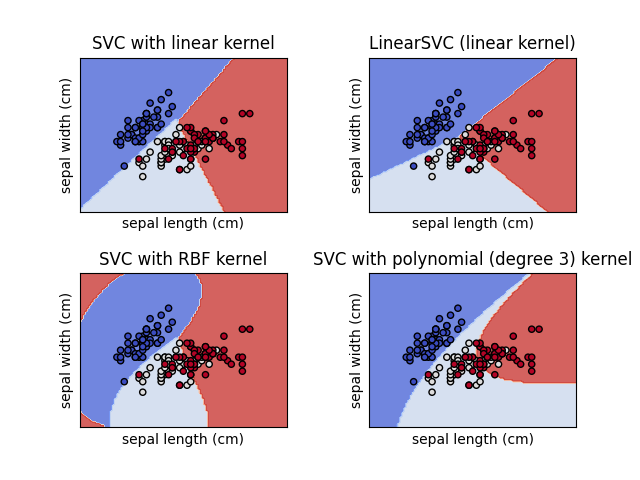
Decision boundaries of SVM models on the Iris dataset.

And this is the correlation matrix between the four models as well as their absolute accuracy.

Correlation of four SVM model predictions on the Iris dataset.

We see that the correlation starts at 0.66, but can be as high as 0.98. These models are clearly not independent.

Joint sampling

The alternative to independent sampling, which takes the correlation between classifiers into account and is to take a joint bootstrap sample when computing \(\mathrm{Acc}_1\) and \(\mathrm{Acc}_2\), before taking their difference \(\Delta \mathrm{Acc}\).

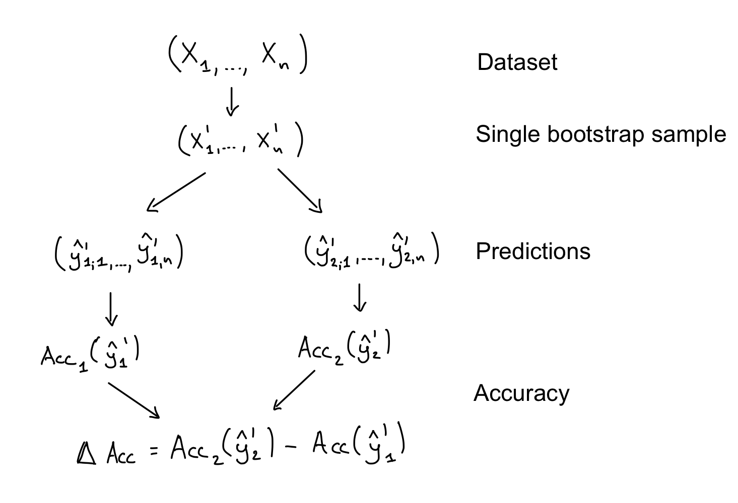
Bootstrapping for \(\Delta \mathrm{Acc}\) via joint sampling.

We first take a single bootstrap sample \(\mathbf{x}'\), and with it we compute

\[\Delta \mathrm{Acc}(\mathbf{x}') = \mathrm{Acc}_2(\mathbf{x}') - \mathrm{Acc}_1(\mathbf{x}')\,.\]

Another way of looking at it is that we treat \(\Delta\mathrm{Acc}(\mathrm{x})\) as a single function of the dataset, regardless of the fact that internally it relies on the predictions of two classifiers.

What is the effect of this change? Let us consider two classifiers with accuracies 75% and 78% and a dataset of size 1,000. Can we be confident that this performance difference is significant? Let us plot the confidence interval for \(\Delta\mathrm{Acc}\) as a function of the correlation for both independent and joint bootstrap sampling.

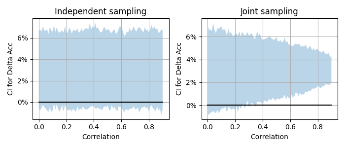
Confidence interval for \(\Delta\mathrm{Acc}\) as a function of the correlation between the classifier predictions.

We see that with joint sampling the confidence intervals become significantly smaller as the correlation increases. This makes sense. The more the two classifiers are correlated, the less uncertainty there is about their relative performance. We still might be uncertain about the absolute performance level, but since we are only interested in comparing them, this correlation comes to our aid.

In particular, we see that with joint sampling any correlation above 0.5 allows us to conclude that the second classifier is indeed better than the first one. A conclusion we would not have been able to make with independent bootstrap sampling.

Minimal detectable change

Another way of looking at the difference between joint and independent sampling is to consider the minimal detectable change in classifier accuracy. We fix the dataset size at \(n=1,000\) and consider a baseline classifier with accuracy of 60%, 70%, 80% and 90% respectively. We ask the following question: How accurate does a second classifier have to be, for us to determine with 95% significance that it is better than the baseline classifier?

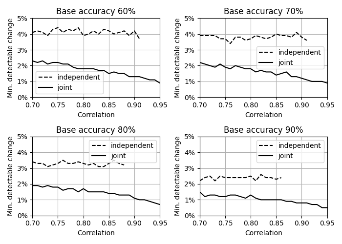
Minimal detectable change in classifier accuracy as a function of correlation for joint and independent sampling.

This graph shows the answer as a function of the correlation between the two classifiers. As the correlation increases, with joint sampling, the mimimal detectable change decreases to below 1% accuracy difference. At the same time, with independent sampling the minimal detectable change does not depend on the correlation.

Conclusion

If we compare ML models and ignore the correlation between them, we give up a lot of discriminative power. The size of the minimal detectable effect increases significantly. We might be forced into ignoring correlation, if we evaluate the two models on different datasets. But, if we can avoid this situation, e.g., by restricting our evaluation on a common subset, we might gain more discriminative power than we lose by reducing the dataset size.

Bootstrapping, while a powerful tool, needs to be tweaked to each individual application. A one-size-fits-all is rarely optimal or even appropriate. But, if used correctly, it allows us to do a lot.

Code

The analysis was done in this notebook using the score-analysis package.