A Journey Along the ImageNet Leaderboard: Transformers
This post is the first of a (planned) series that looks at the papers from the ImageNet leaderboard. As the top places are occupied by Transformers and EfficientNets, we will start our exploration with the 17th place – An Image is Worth 16x16 Words: Transformers for Image Recognition at Scale – the first paper on visual transformers.
Why is this paper important?
We thought that CNNs were successful in computer vision tasks because the model architecture encoded essential properties such as locality and translation-invariance. This seems not to be the case. A visual transformer breaks the image up in patches, flattens them and then treats each patch as a vector of numbers without any a priori knowledge of spatial structure. The trade-off is that more training data is needed—the models are trained on the JFT-300 dataset, consisting of 300M images. It is another example of Sutton’s Bitter Lesson showing that more general methods together with computation and data outperform more specialised and more hand-crafted methods. In the authors’ own words
This result reinforces the intuition that the convolutional inductive bias is useful for smaller datasets, but for larger ones, learning the relevant patterns directly from data is sufficient, even beneficial.
What is a visual transformer?
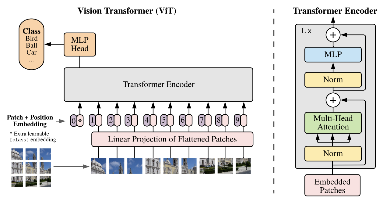
The transformer architecture was first proposed for NLP in the paper Attention Is All You Need. This paper uses the least amount of modifications to apply the architecture to image classification. A 2D image with \(224 \times 224 \times 3\) pixels is split into \(14^2\) patches of size \(16 \times 16 \times 3\) and represented as \(x_p \in \mathbb R^{196 \times 768}\), a sequence of 196 tokens of dimension 768. Next, each token is mapped via a learnable linear projection from \(\mathbb R^{768}\) to \(\mathbb R^D\). The latent vector size \(D\) will stay constant throughout the transformer layers. Values used for \(D\) in this paper are \(768\), \(1024\) and \(1280\). We prepend one more token, \(x_{\mathrm{class}}\), which will, at the output of the network, serve as the image representation and we add a learnable positional embedding, so the final representation is \(z_0 \in \mathbb R^{(N+1) \cdot D}\) with \(N=196\). This is summarized by the formula
\[z_0 = [x_{\mathrm{class}}; x^1_p E; \dots; x^N_p E] + E_{\mathrm{pos}}\,,\]where \(x_{\mathrm{class}} \in \mathbb R^D\), \(E \in \mathbb R^{768 \times D}\) and \(E_{\mathrm{pos}} \in \mathbb R^{(N+1) \cdot D}\) are learnable parameters.

Fig. 1 in the paper.
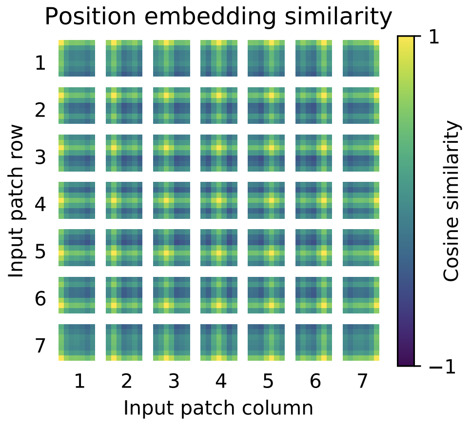
The embeddings are now mapped by \(L\) transformer layers, each of which consists of a multi-head attention block, followed by a multi-layer perceptron (MLP), i.e., two dense layers with a GELU non-linearity in-between. Layernorm is used as the normalization layer. While a visual transformer has less inductive bias than a CNN, it is not completely bias-free. By splitting the image into connected patches locality is to some extent preserved. And the positional encoding preserves some large-scale information about the relative position of patches. In fact, the image below shows that the transformer learns the 2D structure of patches in the positional encoding.

Fig. 7 in the paper.
A visual transformer may appear similar to a visual bag of words model, such as BagNet. However, while the MLP layers act on each patch independently, the attention blocks model interactions between patches. This is contrast to bag of words models, which treat patches independent of each other.
Some training details
The models are trained with the Adam optimizer and a large batch size of 4096. The weight decay at 0.1 is surprisingly large, this apparently helps with transfer learning afterwards. An exponential moving average with weight 0.9999 over trainable parameters is used for the final inference model (Polyak averaging).
How big are these models?
There are different ways to quantify the size of a model: number of parameters, inference speed, number of FLOPS for inference, memory consumption. Unfortunately, the authors only provide inference speed on the TPUv3 architecture and they don’t provide the number of FLOPS. It is of course true that other factors, such as memory access speed and caching, besides the number of FLOPS influence inference speed. However, the number of FLOPS does provide some idea, how different model types compare. So, I wrote a notebook to estimate the number of FLOPS for the vision transformer models of this paper.
| #Parameters | #FLOPS | TPUv3 inference (img/sec) | |
|---|---|---|---|
| EfficientNet-B0 | 5.3M | 0.4B | |
| EfficientNet-B7 | 66M | 37B | |
| ViT-B/16 | 86M | 35.2B | 900 |
| ViT-L/16 | 307M | 123.2B | 300 |
| ViT-H/14 | 632M | 334.8B | 90 |
The models are big… No surprise there. The question is, how fast is inference on CPUs? Can we expect to see vision transformer models used for applications such as face recognition?