Calibration of Neural Networks
This post what it means to calibrate the outputs of neural networks, i.e., to connect the confidence scores that are the result of the training process with probability estimates for the likelihood that the network is making an error. The exposition largely follows the paper by Guo et al. 2017.
1. Introduction
We look at the problem of supervised multi-class classification with neural networks. A network \(f\) is given an input \(x\) and produces \((\hat y, p) = f(x)\), a prediction \(\hat y \in \{1, \dots, K \}\) and a confidence \({p \in [0, 1]}\). Given the true label \(y\) we can check whether the label \(\hat y\) is correct or not and compute the accuracy of the model on a dataset. But how are we to interpret the confidence score?
We will adopt a probabilistic view of the problem: the input \(X \in \mathcal X\) and the labels \(Y \in \{1, \dots, K \}\) are random variables with joint distribution \(\pi(X, Y)\) and the network is a function \((\hat Y, P) = f(X)\).
2. Calibrated Models
A necessary condition. Intuitively, we expect the network to be more accurate on samples with a higher confidence score and less accurate on samples with a lower confidence score. We can formulate the condition like this: for any two confidence scores \(p_1 \geq p_2\) we want the inequality
\[\mathbb P\left(\hat Y = Y \,|\, P \geq p_1\right) \geq \mathbb P\left(\hat Y = Y \,|\, P \geq p_2\right)\]to hold. Note that confidence cannot be interpreted on the level of an individual sample. For each single example the network is either correct or not, there is no more or less confident here. To talk about confidence we need to consider collections of samples. Then we can ask whether on a set of samples with a high confidence score the network is more accurate than on a set with low confidence.
Perfect calibration. The majority of NNs will fulfil this property. Indeed, it would be very remarkable to find a network, trained with cross-entropy, that violates this inequality. But we still do not know how to interpret the numerical value of the confidence score. How does a confidence score of 0.8 compare with 0.9 or even 0.99? To answer this we need to introduce the concept of calibration. We call the confidence scores calibrated, if they accurately represent the probability of the network being correct. We write this as
\[\mathbb P\left( \hat Y = Y \,|\, P = p \right) = p\,, \ \ \ \ \ (1)\]and want this to hold for all \({p \in [0, 1]}\). We call this perfect calibration. In practice, with only finitely many samples, this condition is impossible to achieve, because \({P}\) is a continuous random variable.
Empirical calibration. Instead we need to approximate it. Given \({n}\) samples \({x_1, \dots, x_n}\), we group them into \({M}\) bins and look at the relationship between the accuracy and confidence scores in each bin. Let \({B_m}\) the set of indices of samples whose prediction confidence falls into the interval \({I_m = (\tfrac{m-1}{M}, \tfrac{m}{M}]}\). The accuracy of the classifier on \({B_m}\) is
\[\displaystyle \operatorname{acc}(B_m) = \frac{1}{|B_m|} \sum_{i \in B_m} \mathbf{1}\left(\hat y_i = y_i\right)\,,\]| which is an approximation to—statistically speaking an unbiased and consistent estimator—the probability $${\mathbb P\left( \hat Y = Y \, | \, P \in I_m \right)}\(. The average confidence in bin\){B_m}$$ is |
As an empirical version of perfect calibration (1) we say that the confidence scores are calibrated if
\[\operatorname{acc}(B_m) = \operatorname{conf}(B_m) \,,\quad m = 1, \dots, M\,.\]Note that this notion of calibration depends on our choice of subdivisions \({I_m}\). Uniform subdivisions are a natural choice, but for very accurate models most confidence scores will be close to 1 and so a logarithmic scale \({I_m = [1-10^{-m+1}, 1-10^{-m}]}\) together with a suitable cutoff \({I_M = [1-10^{-M}, 1]}\) might be more appropriate.
3. Measuring Miscalibration
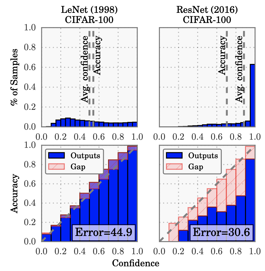
Reliability diagrams. We can represent this condition visually by plotting accuracy against confidence in a reliability diagram such as shown the second row of the following figure. Note that the reliability diagram does not show how many samples fall in each bin and hence does not tell us anything about what proportion of samples is well calibrated.

Confidence histogram and reliability diagrams for two networks. Source: Guo et al. 2017.
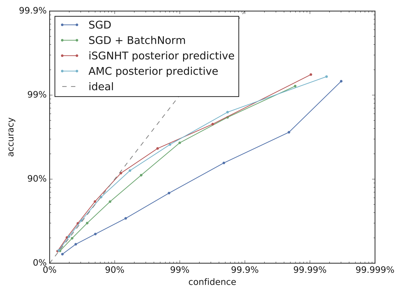
When models become more accurate, as e.g. the ResNet model in the above figure, it may more illuminating to plot both the reliability diagram on logarithmic axes. The next figure from Heek, Kalchbrenner 2019 is an example of this.

Logarithmic reliability diagram for ImageNet classification. Source: Heek, Kalchbrenner 2019.
Expected calibration error. While a visual tool is useful, sometimes it is more convenient to have a scalar summary statistic of calibration. One such statistic is the average difference between accuracy and confidence, i.e.
$$\displaystyle \mathbb E_{p \sim P} \left[ \left| \mathbb P\left(\hat Y=Y \,|\, P=p\right) - p \right| \right]\,. $$
The expected calibration error (ECE) approximates this quantity by partitioning confidence scores into \({M}\) bins as before,
$$\displaystyle \operatorname{ECE} = \sum_{m=1}^M \frac{|B_m|}{n} \left| \operatorname{acc}(B_m) - \operatorname{conf}(B_m) \right|\,. \ \ \ \ \ (2)$$
Other choices of weights in \({\operatorname{ECE}}\). As we are taking the expectation we have a choice, how we weight various parts of the space. In the above definition we use the distribution of confidence scores to weight the integral/sum. This means that if most confidence scores are above 0.9 as can be seen in the right column of Fig. 1, then ECE will be dominated by the difference between accuracy and confidence on that last bin. The differences in the other bins will be of almost no consequence.
If we want the summary metric to reflect the calibration across the whole interval \({[0, 1]}\), we should weight each part of the confidence space equally, i.e., with \({U}\) denoting the uniform distribution on \({[0, 1]}\), we should use
$$\displaystyle \mathbb E_{p \sim U} \left[ \left| \mathbb P\left(\hat Y=Y \,|\, P=p\right) - p \right| \right]\,, $$
and its approximation
$$\displaystyle \operatorname{ECE_{unif}} = \sum_{m=1}^M \frac{|I_m|}{n} \left| \operatorname{acc}(B_m) - \operatorname{conf}(B_m) \right|\,. $$
In some applications the bins we have chosen are a relevant unit of measurement and we want to give each bin an equal weight. This can be the case, e.g. for the logarithmic bins \({I_m = [1 - 10^{-m+1}, 1-10^{-m}]}\) in which case \({|I_m| = 9 \cdot 10^{-m+1}}\) and the bins closer to \({1}\) are getting smaller and smaller. With equal weighting the average calibration error is
$$\displaystyle \operatorname{ECE_{bin}} = \frac 1n \sum_{m=1}^M \left| \operatorname{acc}(B_m) - \operatorname{conf}(B_m) \right|\,. $$
4. Confidence for Imbalanced Datasets
All the above definitions of the calibration error are based on the concept of accuracy. For balanced datasets such as MNIST or ImageNet this makes sense. However, when the classes are unbalanced, this measure will—regardless of the weighting scheme—be dominated by the confidence scores of the larger class(es).
Fraud detection. Let us consider fraud detection as an example of a binary classification problem with imbalanced classes. The model \({f}\) returns a score \({q = f(x)}\) and we classify it based on a threshold \({q_0}\) as \({\hat y = \mathbf{1}(q \geq q_0)}\). We use the labels \({y=1}\) for genuine samples and \({y=0}\) for fraudulent samples.
In a typical application—by typical I mean that I made up some numbers—we would expect less than 5% of all samples to be fraudulent and a common expectation for a fraud detection algorithm is to have a false acceptance rate (FAR) below 1% and a false rejection rate (FRR) below 10%. To put this into formulas we have
$$\displaystyle \begin{array}{rcl} \mathbb P(Y = 0) &<& 0.05 \\ \mathbb P(\hat Y = 1 \,|\, Y = 0) &<& 0.01 \\ \mathbb P(\hat Y = 0 \,|\, Y = 1) &<& 0.1\,. \end{array} $$
Accuracy. In essence, a model is calibrated if the confidence score is representative of the accuracy of the model for samples with that confidence score. But for unbalanced datasets, e.g. when \({\mathbb P(Y=0) \ll \mathbb P(Y=1)}\), accuracy is not a useful performance measure, because its value is mostly determined by the majority class as can be seen by the following calculation
$$\displaystyle \begin{array}{rcl} \operatorname{acc} &=& \mathbb P(\hat Y=Y) \\ &=& \mathbb P(\hat Y=0 \,|\, Y=0)\, \mathbb P(Y=0) + \mathbb P(\hat Y=1 \,|\, Y=1)\, P(Y=1) \\ &=& 1 - \mathbb P(\hat Y=1 \,|\, Y=0)\, \mathbb P(Y=0) - \mathbb P(\hat Y=0 \,|\, Y=1)\, \mathbb P(Y=1) \\ &=& 1 - \mathrm{FAR} \cdot \mathrm{NR} - \mathrm{FRR} \cdot \mathrm{PR} \end{array} $$
Because in fraud detection the negative rate \({\mathrm{NR}}\) is small and because we expect the \({\mathrm{FAR}}\) of the model to be small, it follows that the accuracy will be dominated mostly by the product \({\mathrm{FRR} \cdot \mathrm{PR}}\) of \({\mathrm{FRR}}\) with the positive rate \({\mathrm{PR}}\).
What to do instead? What then shall we do in place of calibration to obtain interpretable scores from our model? One option is to align the confidence score with the false acceptance rate. Let \({\mathrm{FAR}(q)}\) we the false acceptance rate for classification threshold \({q}\), i.e.,
$$\displaystyle \mathrm{FAR}(q) = \mathbb P(Q \geq q \,|\, Y = 0)\,. $$
We say the model is FAR-calibrated, if
$$\displaystyle \mathrm{FAR}(q) = 1 - q\,, $$
or, since \({\mathrm{FAR} + \mathrm{TRR} = 1}\), in terms of the true rejection rate,
$$\displaystyle \mathrm{TRR}(q) = q\,. $$
In other words, we can interpret the decision threshold as the TRR of the model.
How can we FAR-calibrate a model? The relationship between a threshold and the FAR is monotone decreasing—a higher threshold implies a lower FAR and vice versa with the boundaries \({\mathrm{FAR}(0) = 1}\) and \({\mathrm{FAR}(1) = 0}\)—and we can transform the score via
$$\displaystyle P = 1 - \mathrm{FAR}(Q)\,. $$
Then the following two inequalities are equivalent
$$\displaystyle Q \geq q \;\Leftrightarrow\; \mathrm{FAR}(Q) \leq \mathrm{FAR}(q) \;\Leftrightarrow\; P \geq p\,. $$
Thus, if we use \({P}\) instead of \({Q}\) for classification we obtain
$$\displaystyle \begin{array}{rcl} \mathrm{FAR}(p) &=& \mathbb P(P \geq p \,|\, Y = 0) \\ &=& \mathbb P(Q \geq q \,|\, Y = 0) = \mathrm{FAR}(q) = 1 - P\,, \end{array} $$
thus showing that using \({P}\) gives an \({\mathrm{FAR}}\)-calibrated model.
Is this sufficient? There is no final answer to the calibration problem. For applications where false acceptance and false rejection carry different risks, calibration is probably not the right notion, because it hides errors of the minority class.
Regarding alternatives for binary classification, the notion of FAR-calibration only concerns itself with the false acceptance rate and makes no statement about the false rejection rate. Of course we could in the same fashion derive the concept of FRR-calibration and then we would have to make a choice: Do we calibrate the confidences with respect to FAR or FRR? We cannot do both and it is the application that will have to tell us which one to use. For fraud detection, FAR is probably the right choice, because we want to control the amount of missed fraud.